Tsirelson’s bound

Boris Tsirelson

Boris Tsirelson (or Cirel’son, or Цирельсон, or צְיךרלסון) is an Israeli (born Russian) mathematician currently at Tel-Aviv university. Here is the picture from his Wikipedia entry: he has such an incredible stare, he irresistibly reminds me of Orson Welles (picture below). Two great magicians!

Tsirelson worked on the mathematical foundations of nonlocality in the early 80s, at a time when Aspect hadn’t yet realized his conclusive experiments, and the philosophical implications of the EPR paradox and Bell’s work were still being debated (well, they still are even today…). As we saw in the previous post, 20 years earlier Bell had demonstrated that the set of “entangled distributions” — bipartite distributions on pairs of outcomes that can be obtained by measuring spatially isolated quantum systems — was strictly larger than the set of “classical distributions”, i.e. convex combinations of product distributions. Furthermore, Clauser, Horne, Shimony and Holt had discovered a simple inequality that paved the way for the experimental demonstration of that fact; we phrased that inequality as a simple two-player “nonlocal game”.

Orson Welles

Together with their inequality, Clauser et al. described a simple quantum strategy using entanglement (in the following I will refer to strategies for quantum players as “entangled strategies”) that beat the best possible classical strategy by a noticeable amount. Precisely (as we will show) the optimal success probability of classical players is ${75\%}$ , while entangled players can achieve at least ${85\%}$ . Quite surprisingly, it seems that Tsirelson, 10 years later, was the first to ask the obvious question: had CHSH determined the optimal entangled strategy in their game? [10/14 edit: the question was first asked to Tsirelson by A. Vershik] Or could there be an even better one? Could entangled players win the CHSH game with probability ${1}$ ?

Tsirelson answered that question in his first paper on quantum information. In that paper Tsirelson initiated the study of the limitations of entangled strategies: what restrictions are there on the kinds of distributions that can arise from performing local measurements on spatially isolated quantum systems? An obvious limitation is that, if quantum mechanics is to respect special relativity, the distribution must be no signalling: outcomes obtained when measuring one system cannot depend on the choice of measurement made for the other. But are there any other restrictions?

In this post I will first describe some of the more general results in Tsirelson’s paper, as this will give us a chance to introduce the mathematical formalism used to describe entangled strategies — a formalism I expect to use frequently here. I will then describe Tsirelson’s elegant proof of his bound on the maximum success probability of entangled players in the CHSH game. It is a very simple and elegant proof, and an excellent warm-up for the “rigidity” theorem that I will write about in a later post. Moreover, to this day the technique developed by Tsirelson in proving his bound is arguably the only general technique we have to upper bound the success probability of entangled players in a given game! So it is well worth studying in detail.

1. Tsirelson’s 1980 paper

Tsirelson’s paper “Quantum generalizations of Bell’s inequality” contains three main theorems (in fact four, but I admit I can’t really parse the fourth one) — none of which is given a proof! (See this page for more.) For our purposes, the key points are already stated in the first theorem, for which a proof is well-known 🙂 To phrase it in a modern language, this theorem gives a precise mathematical characterization of the set of all possible entangled strategies, i.e. strategies achievable by quantum players using entanglement, in so-called “XOR games”. XOR games are the class of games, such as the CHSH game, in which the players always answer with a single ${0/1}$ bit each, and the validity of a given pair of answers only depends on their parity.

Tsirelson’s characterization is the source of almost all our knowledge about XOR games, which are essentially the only class of two-player entangled games for which we know anything at all (I am probably offending a number of people working hard on the topic — including myself — by saying this!) Before describing this characterization, let’s first review how entangled strategies are modeled in quantum mechanics.

1.1. Entangled-player strategies

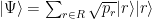
Quantum players in a nonlocal game play as follows. The players start the game in a state (i.e. a unit vector) ${|\Psi\rangle\in{\mathbb C}^d\otimes {\mathbb C}^d}$ , where each copy of ${{\mathbb C}^d}$ represents either player’s share of the state and ${d}$ is an arbitrary integer. Upon receiving her question ${x}$ , Alice measures her share of ${|\Psi\rangle}$ , obtaining an outcome ${a\in\{0,1\}}$ that she sends back as her answer. Her measurement is given by a pair of ${d}$ -dimensional orthogonal projections ${A_x^0,A_x^{1}}$ that sum to identity: ${A_x^0+A_x^{1}=\textrm{Id}_{{\mathbb C}^d}}$ . Similarly, for ever ${y}$ Bob has orthogonal projections ${B_y^0,B_y^{1}}$ . Finally, the only rule we need is the measurement rule (or, to be pedantic, “Born rule”). This rule states that the probability that Alice and Bob obtain oucomes ${a}$ and ${b}$ respectively, when their questions are ${x}$ and ${y}$ , is given by

$\displaystyle p(a,b|x,y)=\langle\Psi| A_x^a \otimes B_y^b |\Psi\rangle.$

That’s all we need to know! A quick sanity check: ${p(a,b|x,y)\geq 0}$ follows since ${A_x^a,B_y^b\geq 0}$ , and ${\sum_{a,b} p(a,b|x,y) =1 }$ follows from the “sum to ${\textrm{Id}}$ ” constraints.

Classical strategies are obtained in the special case ${d=1}$ . Then necessarily one of ${A_x^0}$ , ${A_x^{1}}$ must be ${(1)}$ , the other ${0}$ , and ${p(a,b|x,y)}$ is ${1}$ if and only if ${(a,b)}$ are such that ${A_x^a = B_y^b = (1)}$ . One can also model strategies using shared randomness in this way: if ${(p_r)}$ is a distribution on random strings ${r\in R}$ , and Alice (resp. Bob) answers ${a(x,r)}$ (resp. ${b(y,r)}$ ) on question ${x}$ (resp. ${y}$ ) and random string ${r}$ , define ${|\Psi\rangle = \sum_{r\in R} \sqrt{p_r} |r\rangle|r\rangle}$ , and let ${A_x^a}$ be the ${|R|}$ -dimensional diagonal matrix with ${(A_x^a)_{r,r} = 1}$ if ${a(x,r)=a}$ , and ${0}$ otherwise. Then one can check that ${p(a,b|x,y)}$ as defined above is ${\sum_{r: a(x,r)=a,b(y,r)=b} p_r }$ , as it should be. Hence it is sometimes fruitful to think of entangled strategies as a non-commutative generalization of classical randomized strategies.

1.2. Tsirelson’s characterization

Suppose given a strategy ${\{A_x^a\}}$ , ${\{B_y^b\}}$ , ${|\Psi\rangle}$ for players in an XOR game ${G}$ . An important observation is that the players’ success probability in the game only depends on the differences ${A_x:=A_x^0-A_x^{1}}$ , ${B_y:=B_y^0-B_y^{1}}$ . Indeed, for any question ${(x,y)}$ , either answers with parity ${0}$ or answers with parity ${1}$ will be accepted. Hence to ${G}$ we can associate a function ${f_G(x,y)\in\{0,1\}}$ describing the correct parity for the pair of questions ${(x,y)}$ . Using ${\textrm{E}_{x,y}}$ to denote the expectation over the choice of a pair of questions ${(x,y)}$ in ${G}$ , the player’s success probability is

$\displaystyle \begin{array}{rcl} \textrm{E}_{x,y} \sum_{a,b: a\oplus b = f_G(x,y)} p(a,b|x,y) &=& \textrm{E}_{x,y} \sum_{a,b} (-1)^{f_G(x,y)}\frac{((-1)^{a\oplus b}+(-1)^{f_G(x,y)})}{2} p(a,b|x,y)\notag\\ &=& \frac{1}{2} + \frac{1}{2}\textrm{E}_{x,y} (-1)^{f_G(x,y)} \sum_{a,b}(-1)^{a\oplus b}p(a,b|x,y), \end{array}$

and in the case of entangled strategies, by the Born rule the last sum evaluates to ${\langle\Psi| A_x \otimes B_y |\Psi\rangle}$ . In general, ${A_x}$ , ${B_y}$ are arbitrary Hermitian matrices that square to identity; any such matrices are called “observables” in quantum mechanics.

Fix an XOR game ${G}$ , and let ${X}$ (resp. ${Y}$ ) denote the set of possible questions to Alice (resp. Bob). Tsirelson’s first theorem states that, given a set of observables ${\{A_x\}}$ and ${\{B_y\}}$ and a state ${|\Psi\rangle}$ , there exists another set of observables ${\{\hat{A}_x\}}$ , ${\{\hat{B_y}\}}$ of dimension ${\hat{d}\leq \max(2^{\lceil|X|/2\rceil},2^{\lceil|Y|/2\rceil})}$ , such that for every ${x,x'}$ the anti-commutator ${\hat{A}_x\hat{A}_{x'}+\hat{A}_{x'}\hat{A}_x = c_{x,x'}\textrm{Id}}$ for some ${c_{x,x'}}$ , and for every ${x,y}$ ,

$\displaystyle \langle\Psi| A_x\otimes B_y |\Psi\rangle = \langle \hat{\Psi}| \hat{A}_x\otimes \hat{B}_y |\hat{\Psi}\rangle,$

where ${|\hat{\Psi}\rangle}$ is the fixed state ${\sum_i \hat{d}^{-1/2}|i\rangle |i\rangle}$ , such that the strategy ${\{\hat{A}_x\}}$ , ${\{\hat{B}_y\}}$ , ${|\hat{\Psi}\rangle}$ exactlyreproduces the correlations of the original strategy, and in particular achieves exactly the same success probability in the game ${G}$ . (In fact, the construction of ${\{\hat{A}_x\}}$ and ${\{\hat{B}_y\}}$ only depends on ${G}$ through the sizes ${|X|,|Y|}$ , and the same strategy will reproduce the original correlations in any XOR game of the same size as ${G}$ .)

Tsirelson’s characterization simplifies the strategy in two important respects: first, the dimension is bounded ( ${\hat{d}}$ is independent of ${d}$ ), and second the players’ state is fixed ${(|\hat{\Psi}\rangle}$ is called the “maximally entangled” state in ${\hat{d}}$ dimensions; in a certain precise sense it is the “maximum entropy” state). There is also the additional condition on the anti-commutators, which as we will see can sometimes be useful. These simplifications are crucial in many applications in which one seeks to characterize the set of entangled strategies.

Tsirelson obtained a further characterization of entangled strategies based on the use of vectors alone (no matrices!). I will not describe this step here, but only mention one important consequence: it implies that the largest possible success strategy of entangled players in an XOR games can be expressed as a polynomial-size (in the number of questions in the game) semidefinite program. In particular, this maximum success probability can be efficiently computed. This is in contrast to the maximum success probability of classical players in such games, which is known to be NP-hard to compute (or even, as follows from the PCP theorem and work by Hästad, to approximate within a constant factor).

2. Tsirelson’s bound on the CHSH game

2.1. Bounding classical strategies

Before proving a limitation on the success probability of quantum strategies in the CHSH game, it may be useful to first write down a formal proof of the bound on classical strategies, and see why this proof fails in the quantum setting. Strategies of classical players are easy to describe: for each possible question ${x}$ , Alice has an answer ${a_x\in\{0,1\}}$ , and similarly Bob has an answer ${b_y\in\{0,1\}}$ to each of his possible questions ${y\in\{0,1\}}$ . In what follows it will be convenient to use the notation ${A_x = (-1)^{a_x}}$ and ${B_y = (-1)^{b_y}}$ . For such a strategy it is clear that the probabilities ${p(a,b|x,y)}$ satisfy

$\displaystyle \sum_{a,b} (-1)^{a\oplus b} p(a,b|x,y) \,=\, A_x B_y.$

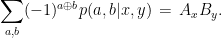
Going back to the expression we gave above for a given strategy’s success, the players’ probability of winning in the CHSH game is exactly

$\displaystyle \begin{array}{rcl} \frac{1}{2}+\frac{1}{8}\big( A_0B_0 + A_1 B_0 + A_0 B_1 - A_1 B_1\big) &=& \frac{1}{2}+\frac{1}{8}\big( A_0 (B_0 + B_1) + A_1 (B_0 - B_1)\big)\\ &\leq&\frac{1}{2}+\frac{1}{8}\big( |B_0 + B_1| + |B_0 - B_1|\big)\\ &\leq& \frac{3}{4}. \end{array}$

Note the magic that happened in the last step: while a trivial bound would have ${|B_0 + B_1| + |B_0 - B_1|\leq 4}$ , we used the fact that, given two numbers in ${\{\pm 1\}}$ , exactly one of their sum or their difference must equal ${0}$ , and the other ${2}$ . Note however that this is wrong for “non-commuting numbers”, i.e. matrices! Take for instance

$\displaystyle B_0 = \begin{pmatrix} 1 & 0 \\ 0 & -1 \end{pmatrix}\quad\text{and}\quad B_1 = \begin{pmatrix} 0 & 1 \\ 1 & 0 \end{pmatrix}.$

Then ${B_0}$ and ${B_1}$ both have operator norm ${1}$ (they are observables, i.e. Hermitian and square to identity), but ${\|B_0+B_1\|_\infty = \|B_0-B_1\|_\infty = \sqrt{2}}$ , so ${\|B_0 + B_1 \|_\infty + \|B_0 - B_1\|_\infty = 2\sqrt{2}}$ , a factor ${\sqrt{2}}$ larger than the best possible in one dimension…

2.2. Bounding entangled strategies

On his webpage, Tsirelson affectionately calls his bound “my bound”, and lists roughly a hundred references to his 1980 paper. But he is modest: google scholar finds 583 citations! Better than a hundred words, here is a faithful reproduction of Tsirelson’s original proof of his bound:

To make Tsirelson’s proof match with the notation we have been using, one only need set ${A_i}$ (resp. ${B_j}$ ) in his proof to ${A_{i-1}\otimes \textrm{Id}}$ (resp. ${\textrm{Id}\otimes B_{j-1}}$ ) as used here. Tsirelson’s inequalities are operator inequalities, meaning that they hold when evaluated on any state: the derivation above implies that for any ${|\Psi\rangle}$ , using our notation

$\displaystyle \langle\Psi| A_0\otimes B_0 + A_0 \otimes B_1 + A_1 \otimes B_0 - A_1\otimes B_1 |\Psi\rangle \leq 2\sqrt{2} \langle\Psi| \textrm{Id}\otimes\textrm{Id}|\Psi\rangle=2\sqrt{2}. \ \ \ \ \ (1)$

Plugging this inequality back into the equation describing a given strategy’s success in the CHSH game, one immediately gets that the maximum success probability of any entangled strategy in the CHSH game is at most ${1/2+\sqrt{2}/4 \approx 0.85}$ ; as demonstrated by Clauser et al. this is tight.

Given an inequality, it is always instructive to look at the cases that saturate it: what is required for there to be equality in Tsirelson’s derivation? Asking this question could be the first step in the proof of a “robust” analogue of Tsirelson’s bound, in which one tries to understand the constraints placed on any ${A_i,B_j}$ that obtain a value close to ${2\sqrt{2}}$ in~(1). For instance, we see that for the inequalities to be tight all four squares appearing in the middle of the derivation must be ${0}$ ! This immediately leads to equations relating the ${A_i}$ and ${B_j}$ …

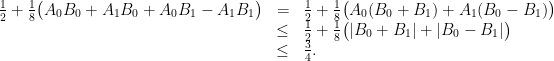
We will pursue this avenue in the next post. I will end this one by giving what I always thought was Tsirelson’s original proof of his bound, and that I don’t know whom to attribute to any more (anyone knows?) [10/14 edit: Boris Tsirelson pointed out this proof appears in a paper by L.J. Landau, “On the violation of Bell’s inequality in quantum theory.” Phys. Lett. A 120:2, 54-56]. The idea is to mimic the proof in the classical setting, taking the square of the left-hand side of (1) instead of attempting to directly use the triangle inequality:

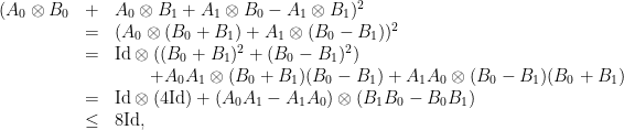
$\displaystyle \begin{array}{rcl} (A_0\otimes B_0 &+ &A_0 \otimes B_1 + A_1 \otimes B_0 - A_1\otimes B_1)^2 \\ &=& (A_0\otimes (B_0+B_1) + A_1 \otimes (B_0-B_1))^2\\ &=& \textrm{Id}\otimes ((B_0+B_1)^2+(B_0-B_1)^2) \\ &&\qquad + A_0A_1\otimes (B_0+B_1)(B_0-B_1) + A_1A_0\otimes (B_0-B_1)(B_0+B_1)\\ &=& \textrm{Id}\otimes (4\textrm{Id}) + (A_0A_1-A_1A_0)\otimes (B_1B_0-B_0B_1)\\ &\leq &8\textrm{Id}, \end{array}$

where we repeatedly used that ${A_x,B_y}$ are observables to write ${A_i^2 = B_y^2 = \textrm{Id}}$ . Taking the square root (which is operator monotone) gives the same result as Tsirelson’s. Once again, all inequalities are operator inequalities, and looking for cases of equality will give us information about the operators achieving near-optimality. For instance, saturating the last inequality requires that both ${A_0}$ and ${A_1}$ , and ${B_0}$ and ${B_1}$ , anti-commute…

12 Responses to Tsirelson’s bound

Boris Tsirelson says:

October 14, 2012 at 7:59 pm

Many thanks, Thomas, for your numerous compliments. (Especially, my face; you are the first…)
“Quite surprisingly, it seems that Tsirelson, 10 years later, was the first to ask the obvious question…” (your post) — “Though, I just answered the question. It was A. Vershik who raised it.” (“my bound”).

- Thomas says:
  
  October 14, 2012 at 9:24 pm
  
  Edited — thanks.
  
Boris Tsirelson says:

October 14, 2012 at 8:14 pm

“I will end this one by giving what I always thought was Tsirelson’s original proof of his bound, and that I don’t know whom to attribute to any more (anyone knows?)” — Yes, I know: 1987 L.J. Landau, “On the violation of Bell’s inequality in quantum theory.” Phys. Lett. A 120:2, 54-56. [MR88b:81019] (see his eq. (1)).

- Thomas says:
  
  October 14, 2012 at 9:17 pm
  
  Ah, many thanks! I edited the post with the reference.
  
Boris Tsirelson says:

October 14, 2012 at 8:35 pm

“contains three main theorems — none of which is given a proof!” — Yes, I feel somewhat guilty. But I was in Soviet Union, in Alya Refusal (not a dissident, but surely not a loyal citizen). In that position it was hard for me to publish anything in Soviet Union (do not forget: no Internet yet…), and even harder to publish outside Soviet Union. This was made illegally; the text was taken by a physicist from abroad, in secret from KGB. But there is also a scientific reason. Now it is probably difficult to believe, but that time such Bell-type matter was considered quite marginal. Also for that reason it was difficult to publish more than a short note.

- Thomas says:
  
  October 14, 2012 at 9:23 pm
  
  Sorry, I certainly did not mean to throw any blame for the absence of proofs…given the current state of publishing practices in computer science I would be in for some work if I did 🙂
  I only briefly tried to find proofs for the main theorems in some of your later papers: have they not appeared at all?
  
  - Boris Tsirelson says:
    
    October 14, 2012 at 10:10 pm
    
    Theorem 1 is proved in: 1985 B.S. Tsirel’son, “Quantum analogues of the Bell inequalities. The case of two spatially separated domains.”
    (Russian) Zapiski LOMI 142, 174-194. [MR86g:81009]
    (English) 1987 Journal of Soviet Mathematics 36:4, 557-570.
    (See Theorem 2.1 there). The translation introduced some (additional?) errors; they are corrected (by hand) here: http://www.tau.ac.il/~tsirel/download/qbell87.html
    The proof was also presented in (one or more) more recent, and more clear, articles. (If you want, I probably can find details.)
    
    Theorems 2 and 3 are long and boring calculations… No, you cannot find a proof in my texts. However, I remember some young person asked me how to do it (at least one of them); and he found a mistake in my formulas; he used computerized symbolic calculations. (If you want, I probably can find details. I can also tell you the idea of the proofs.)
    
Curious Me says:

December 10, 2016 at 5:05 am

Where can I find a proof for Tsirelson’s theorem that d = 2 with the maximally entangled state suffices? I.e. Is there an easy proof for this?

- Thomas says:
  
  December 10, 2016 at 5:18 am
  
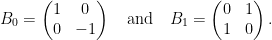
  To show d=2 is sufficient you only need to find a strategy that achieve’s Tsirelson’s dimension in dimension 2. It is not too hard to find. You already know the state should be maximally entangled. I’ll give you Alice’s observables: A_0 = X (Pauli bit-flip) and A_1 = Z (Pauli phase-flip). From here on, finding the best choice of observables for Bob is not hard.
  
  - Curious Me says:
    
    December 11, 2016 at 6:00 am
    
    My question was really more about the following section. I’m trying to find a proof for this:
    
    … such that for every {x,x’} the anti-commutator {\hat{A}_x\hat{A}_{x’}+\hat{A}_{x’}\hat{A}_x = c_{x,x’}\textrm{Id}} for some {c_{x,x’}}, and for every {x,y},
    
    \displaystyle \langle\Psi| A_x\otimes B_y |\Psi\rangle = \langle \hat{\Psi}| \hat{A}_x\otimes \hat{B}_y |\hat{\Psi}\rangle,
    
    where {|\hat{\Psi}\rangle} is the fixed state {\sum_i \hat{d}^{-1/2}|i\rangle |i\rangle}, such that the strategy {\{\hat{A}_x\}}, {\{\hat{B}_y\}}, {|\hat{\Psi}\rangle} exactlyreproduces the correlations of the original strategy, and in particular achieves exactly the same success probability in the game {G}.
    
Thomas says:

December 12, 2016 at 1:00 am

Ah, yes. Tsirelson does have a published proof of that statement, in a later paper. See Theorem 2.1 (and Lemma 1.1 and 1.2 for the construction) here: http://www.tau.ac.il/~tsirel/download/qbell87.pdf

Manmatha Roy says:

May 30, 2019 at 12:07 pm

“what is required for there to be equality in Tsirelson’s derivation?” exactly this proof I needed. How to show that maximally entangled settings with those peculiar basis plays optimally in CHSH